In this post, I give an end-to-end example of using human feedback data to align a diffusion model with direct preference optimization (DPO). If you’d like to test it out or follow along with the code, have a look at the notebook in this repo.
Intro
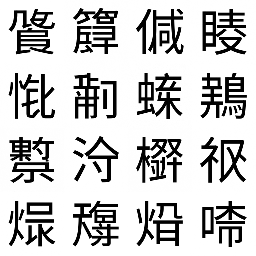
This post builds on my previous glyffuser project, a diffusion model trained to generate novel Chinese-like glyphs. I encountered a common problem in generative AI: low consistency of good generations. While some samples are convincing, others look wrong to anyone who has some experience with Chinese characters. I’ve highlighted some examples in the figure below:
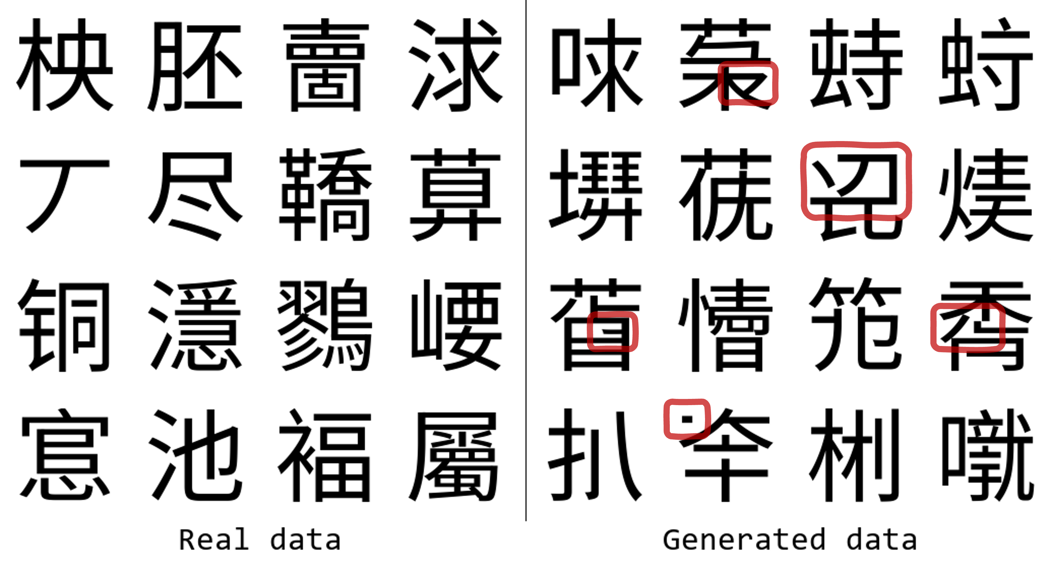
Examples of glyffuser training data (left) and generated data (right); parts that ’look wrong’ are highlighted in red.
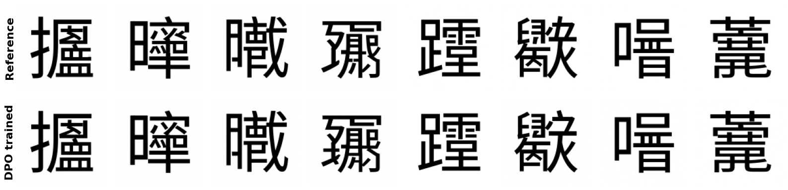
The problem of ‘glyph plausibility’ is difficult to specify computationally, but easy for a human to assess as Chinese characters tend to obey certain stroke order and structural rules. Thus, it presents an good opportunity for post-training model alignment. I’ll go through how to gather preference data from a human “expert” (me), then use DPO to align the model to only produce highly plausible glyphs. A preview of the results below—I think the improvement should be clear, even to the untrained eye! Samples generated by the reference glyffuser model (top) and the DPO-aligned model (below)
Background
Using human feedback to align generative models is the key post-training ‘secret sauce’ that turned text completion models into useful chatbots. OpenAI developed the general-purpose reinforcement learning with human feedback (RLHF) method and used it to create InstructGPT from the base GPT-3 model, paving the way for ChatGPT and the subsequent deluge of LLM-based chatbots. RLHF can also be used to align diffusion models.
A drawback to RLHF is that it is somewhat complicated to implement: a separate “reward model” needs to be trained on human feedback data, and then used to align the base model by assessing its outputs and adjusting its weights accordingly.
Direct preference optimization (DPO) is a streamlined reformulation of RLHF that has become a widely used alternative for human-feedback alignment in models such as Llama 3. It dispenses with the need to train a reward model, instead allowing the model to be directly tuned on paired human preference data. Like RLHF, DPO can also be used to align diffusion models.
Getting human feedback data
To use DPO, we need human feedback data in the form of preference pairs: a pair of samples ranked by a human on some criterion. Here, our samples are pairs of 128×128 pixel images generated by the model. The criterion is simply “which sample is a more plausible Chinese glyph?”
In practical terms, I generated a 10,000 image set using the unconditional glyffuser model (repo, model weights) and (since this is 2025) vibe coded a simple GUI for saving preference data (repo):
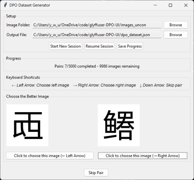
A simple GUI for generating a human preference dataset. Here, those familiar with Chinese characters would almost certainly prefer the example on the right.
The key design choice here was to use keyboard shortcuts to improve ergonomics. I included a skip function as well, to drop one sample where it wasn’t clear which was better. Using the GUI, the process was fairly painless, taking me around 2 hours to label 10,000 pairs (while listening to an audiobook!)
The result was a json file with around 2,500 pairs (around 5,000 samples being dropped) structured in this way:
| |
Implementing the diffusion-DPO loss
While the derivation of the diffusion-DPO loss is nontrivial, the implementation is fairly straightforward, as described in the pseudocode in section S9 of the diffusion-DPO paper:
| |
We can almost paste this code directly into python—see the notebook section “DPO Loss Function” for the exact details.
(Note: since we’re not using text conditioning, we can simply ignore c.)
Below I’ll discuss what’s happening in this loss function; if you’re mainly interested in the implementation, feel free to skip to the next section.
To interpret the DPO loss, we need to recall the standard diffusion training loop for the noise-prediction model (commonly a U-net), the core of a diffusion model. If you aren’t familiar with this, I’ve written a diffusion explainer that goes through this topic clearly with minimal assumed knowledge.
To summarize, in the diffusion training loop we:
- Define a noising trajectory via timesteps, where
t = 0is uncorrupted data andt = 1000is pure (pixel-wise) Gaussian noise. - Take a random training example, and noise it to a random timestep
t. This is efficient as Gaussian noise for anytcan obtained in closed form. - Pass the noised example through the noise-prediction model to obtain predicted noise.
- Update the weights of the noise-prediction model by minimizing the mean squared error (MSE) loss between the predicted noise and actual noise, conditioned on the timestep.
- Repeat. Over many samples and timesteps, the model learns to predict noise for the training data distribution at any given point on the denoising trajectory.
Differences in the diffusion-DPO loss:
- We start with a noise-prediction model pre-trained using the method above.
- We load one copy as a frozen
ref_modeland another as a trainablemodel. - Instead of a single sample as before, each training sample is a preference pair (
x_w,x_l). - We noise both samples with identical noise to obtain
noisy_x_wandnoisy_x_l. - We then pass the noised pair through both models to obtain 4 noise predictions:
model_w_pred,model_l_pred,ref_w_predandref_l_pred. - From these, we obtain 4 MSEs between predicted and actual noise:
model_w_err,model_l_err,ref_w_err, andref_l_err. - We construct the diffusion-DPO loss by combining these errors.
The overall aim of the diffusion-DPO loss is to push model to generate samples more similar to x_w, and less similar to x_l. To do this, we define w_diff and l_diff as the differences between the model error and the reference error. Intuitively, we want to to minimize w_diff while maximizing l_diff. These values are combined in inside_term with a scaling term beta, then passed through a log-sigmoid to generate a log-likelihood loss. The figure belows visualizes this: to minimize the loss, we want to maximize inside_term, which means reducing w_diff and increasing l_diff.
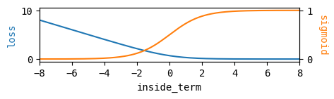
How the DPO loss varies with inside_term
To paraphrase Linkin Park’s “Numb”:
I’m becoming this, all I want to do
Is be more likex_wand be less likex_l
Creating the training script
We can base the diffusion-DPO training script the standard diffusion training script for the glyffuser with relatively small changes:
- Single image data were previously loaded with a standard pytorch
Dataset. Now we create a customPreferenceDatasetthat reads the human feedback JSON created before, and returns an image preference pair. - The training loss was previously a single MSE; we substitute in the diffusion-DPO loss discussed above.
Train the model and assess the results
We can start with the key training hyperparameters from the diffusion-DPO paper:
A learning rate of 2000⁄β 2.048·10⁻⁸ is used with 25% linear warmup. The inverse scaling is motivated by the norm of the DPO objective gradient being proportional to β (the divergence penalty parameter) [33]. For both SD1.5 and SDXL, we find β ∈ [2000, 5000] to offer good performance (Supp. S5). We present main SD1.5 results with β = 2000 and SDXL results with β = 5000.
S5 offers a little more information (recall that β is the coefficient for inside_term):
For β far below the displayed regime, the diffusion model degenerates into a pure reward scoring model. Much greater, and the KL-divergence penalty greatly restricts any appreciable adaptation.
Since our data distribution, preference dataset size and model complexity are all quite different from the paper, I started with runs around the same scale as the base model training—100 epochs of the 2,500 pair dataset (an overnight run on my RTX3090 GPU). An initial run at β = 5000 shows very little change:
Samples generated by the reference glyffuser model (top) and a DPO-aligned model trained at β = 5000 (below). The differences are so small this resembles a ‘spot the difference’ game.
Further testing shows lower β values give better results. The interactive figure below shows output of a training run at β = 1500 over 200 epochs.
While there currently don’t exist any scoring models that can assess ‘glyph plausibility’, the subjective quality change is very clear to me:
- 12 or more of the 16 glyphs from the reference model (epoch 0) have problems
- By 100 epochs, only around half of the glyphs have clear problems and the problems are less pronounced
- At 200 epochs, glyph construction is good but we lose a lot of glyph complexity, likely due to overfitting to the small preference set. (I often favoured simpler glyphs when generating the preference set, as complex glyphs tended to contain more errors.)
At 200 epochs, training metrics were still improving (see figure below) and importantly the preference gap l_diff - w_diff was still increasing. Looking at progression above, however, we can’t rely on metrics and have to make a judgement on when to stop training. Here, I think that 130-150 epochs seems to strike a good balance of creativity and plausibility.
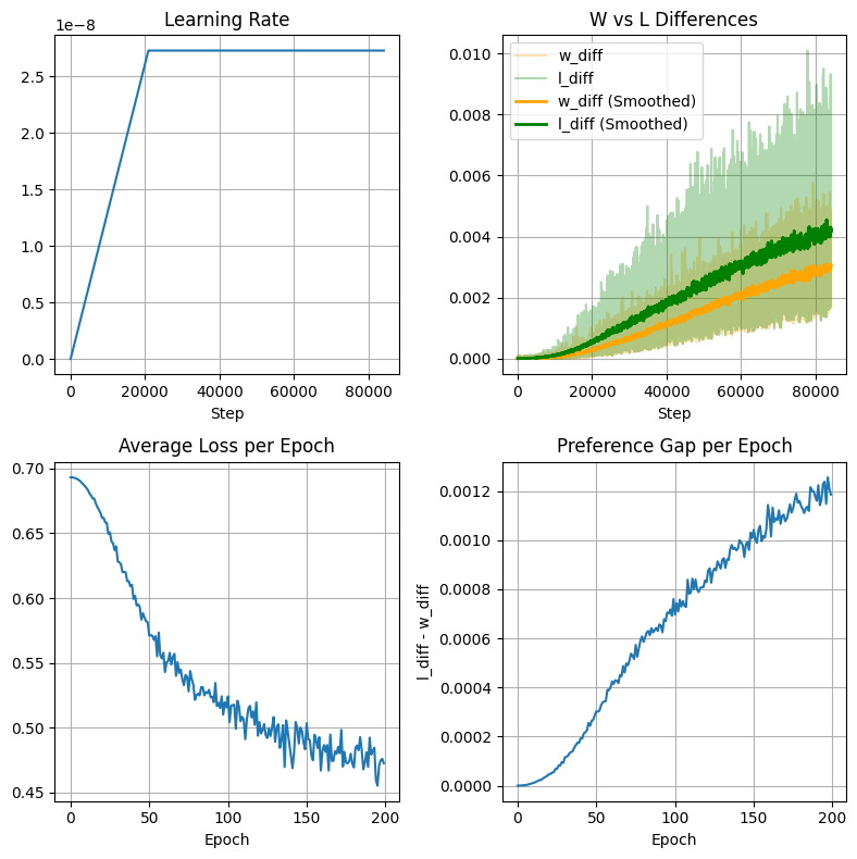
Training metrics for DPO alignment at β = 1500 over 200 epochs.
Further remarks
I hope that if you’re interested using human feedback to align your models but weren’t sure where to start, this has given you some ideas!
I was surprised at how effective the model alignment was with a relatively small dataset. With the increasing interest in diffusion models (and other generative models) in the sciences, this might be an interesting avenue of research. Preference sets might be generated automatically from literature using agentic methods. A brief search reveals only a few papers in this area (example).
DPO alignment also worked for the text-conditioned glyffuser model, but I’ve left that out of this post as I think it complicates things without changing the basic idea.